How to insert a pivot table into a Google Sheet

Google Sheets play an important role in organizing data, however, when you have too much data to manage, it becomes challenging. This is where pivot tables come in. 

In this article, we are going to share a step-by-step guide regarding how you can use the pivot table function of Google Sheets to organize data more effectively. By reading through this article, you will be able to grasp all the basics of pivot tables in Google Sheets. So, let's get started.    

How do I insert a pivot table into a Google Sheet?

If you want to insert a pivot table into a Google Sheet, you don't have to be an expert. All you need is a Google Sheets report editor and some organized data. Once you have the data and the spreadsheets ready, simply follow these steps:

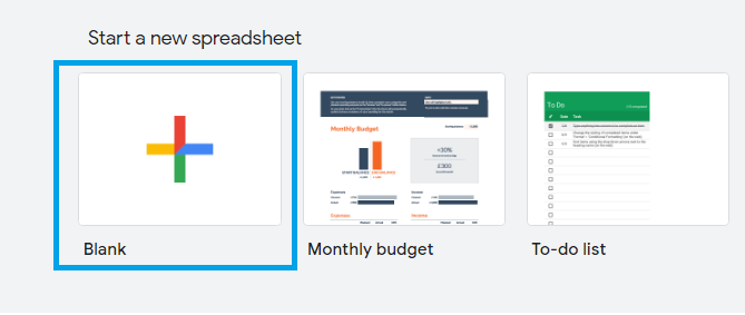
Step 1: First of all, open a new Google sheet spreadsheet

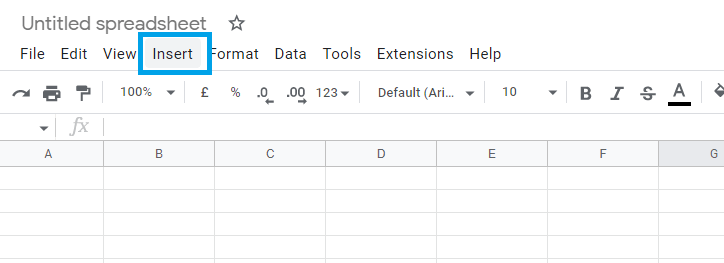
Step 2:  Now Go to the Google sheets menu and click on “Insert”

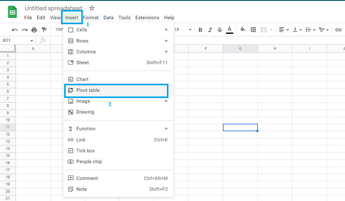
Step 3:  In the “Insert” sub-menu, select the “Pivot table”

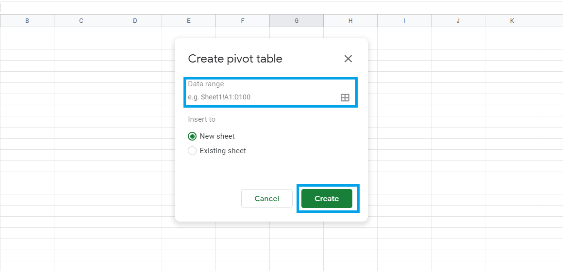
Step 4: On the "Create pivot table" modal that pops up on your screen, enter your data range, select where to insert it, either in a "New sheet" or "Existing sheet," and then click "Create."    In this case, we are going to work with the range: A1:F70.

Step 5:  A Pivot table will be generated automatically 

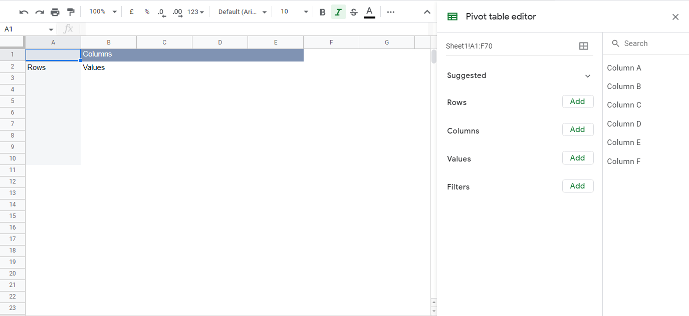You can add rows, columns, data, and filters to the "pivot table editor.".

Conclusion

Ultimately, we learned how to create pivot tables. With pivot tables, you can choose the sorting criteria as you enter data, which will result in your information being sorted and filtered

Keywords: Google Docs, Google Sheet, insert a pivot table into a Google Sheet