How to highlight the negative numbers using Conditional formatting

If you want to make your negative numbers appear red, you can use conditional formatting. By using conditional formatting, you can apply formatting rules based on the cells' values. In this article, we are going to use conditional formatting to highlight all the cells with values less than 0.  

How to highlight the negative numbers using Conditional formatting

To highlight negative integers, follow these steps:

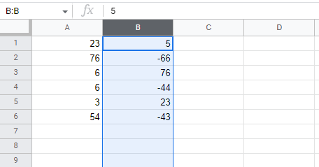
Step 1: On your spreadsheet, select the range of cells that you want to highlight the negative integers. In our case, we are going to work on column B

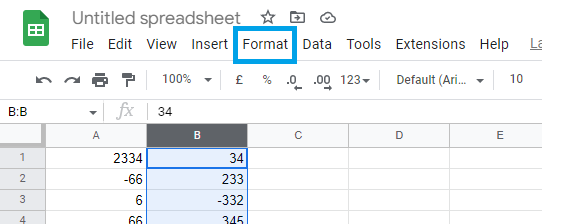
Step 2:  Click "Format" in the Google Sheets menu    

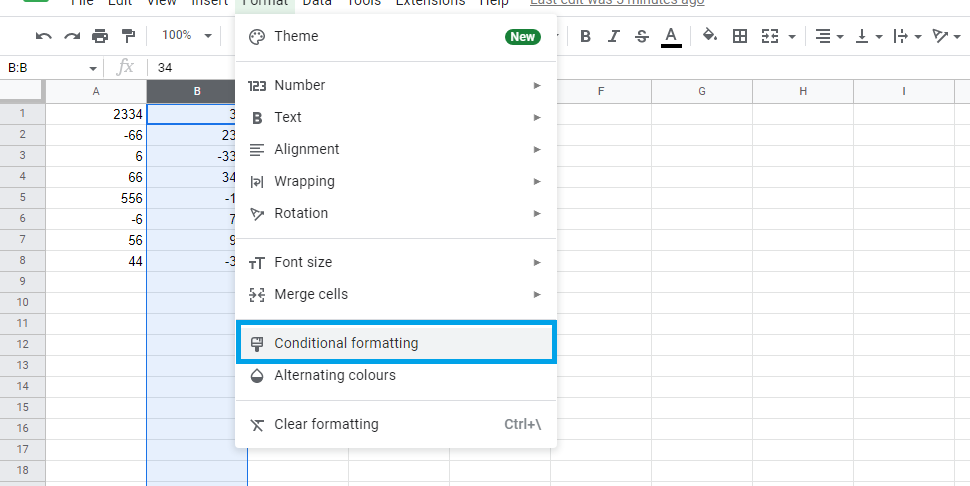
Step 3: Select "Conditional formatting" from the "Format" submenu.

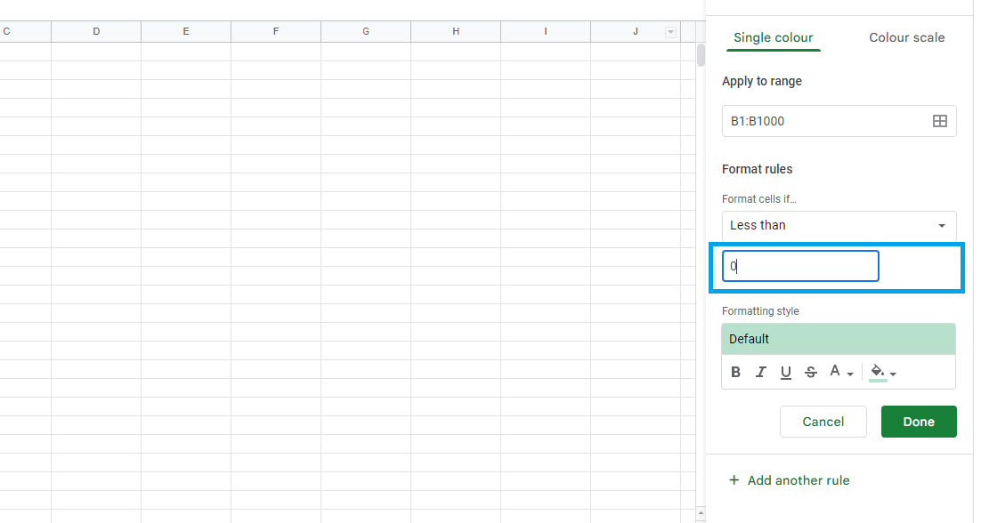
Step 4: On the Format Rules, select “Less than”

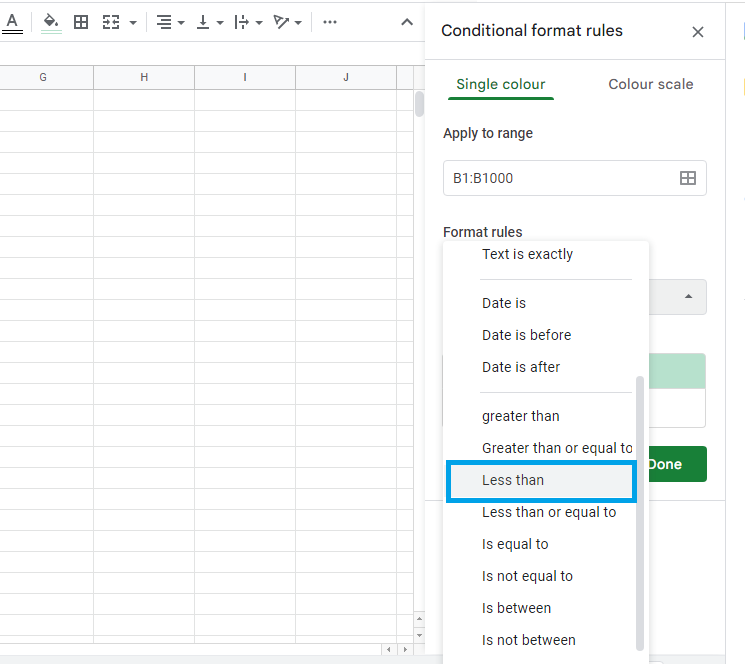Step 5:  In the text box that says “Value or formula” beneath the option you just selected, enter a zero (0)

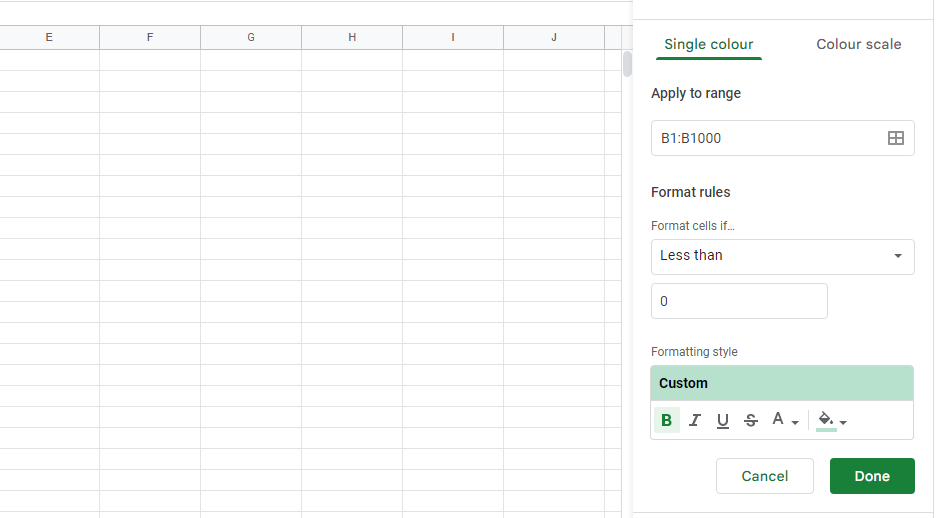
Step 6: Choose your "Formatting style" now. For this case, we are going to bold the negative integers and give the cells a Green background.

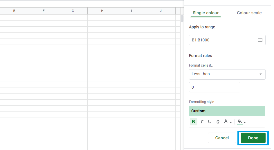
Step 7: Click on the green button “Done.”

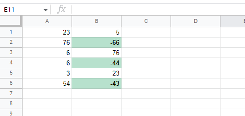
Step 8: The negative integers are now highlighted and easier to see.

Conclusion

In this article, I've shown you how to make your spreadsheet more visible by highlighting all the negatives. When using conditional formatting, you can make the text bold, italic, change font size, change font color, and so on to highlight your negative numbers

Keywords: Google Sheet, Google Docs, How to highlight the negative numbers using Conditional formatting