How to Protect cells using Protect sheets and Ranges in Google Sheets
Protect specific cells in Google Sheets to limit editing access while allowing others to view or comment without altering key data - RRTutors.
You can edit documents in the cloud with anyone with editing permissions with Google Sheets. By disabling editing in a specific cell, you can prevent someone from making changes in that cell without completely removing their editing permissions. This can be achieved using cell protection. In this article, we are going to go through how we can protect formulas in Google sheets
How to Protect cells using Protect sheets and Ranges in Google Sheets
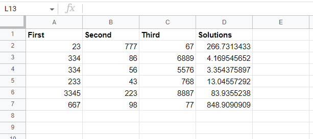
Step 1: Open a Google sheet spreadsheet and select the cells you want to protect.
 |
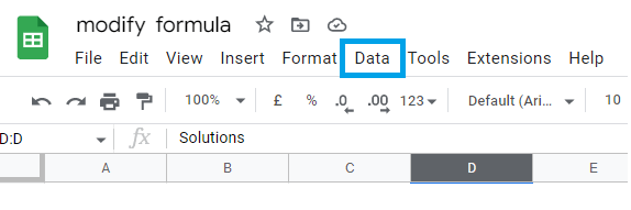
Step 2: Now, on the Google sheets menu, click on “Data”
 |
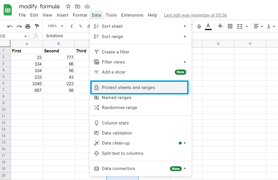
Step 3: On the “Data” submenu, click on “Protect sheets and Ranges”
 |
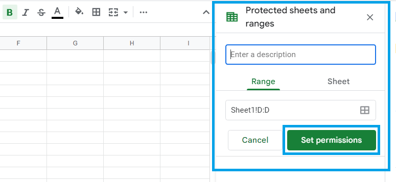
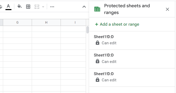
Step 4: In the Protected Sheets and Ranges pane on the right, you can enter a brief description and click "Set Permissions" to customize the cell's protection permissions.
 |
Step 5: By default, anybody with permission to modify the document may alter every cell on the page. To restrict who may edit the chosen cells, use the dropdown option under "Range editing permissions" and then click either "Custom" or “Only you.
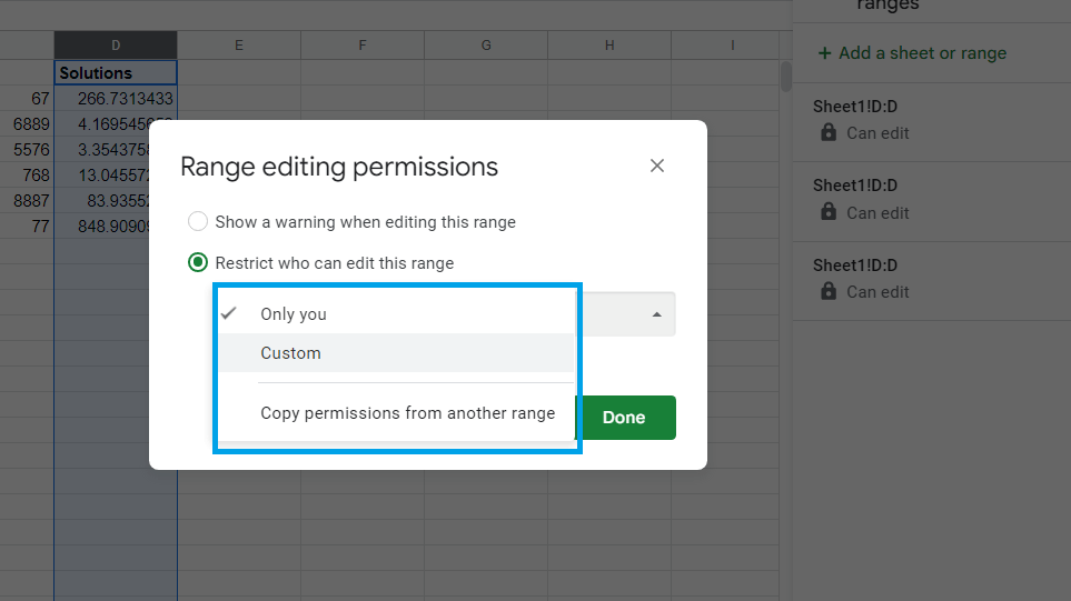 |
If you choose “only you,” it is only you who will be able to edit the selected column; on the other hand, if you choose the “custom” option, then it will be only the selected individuals who will be able to edit the selected cells. In this case, we are going to select “Only you.”
Step 6: Click “Done”
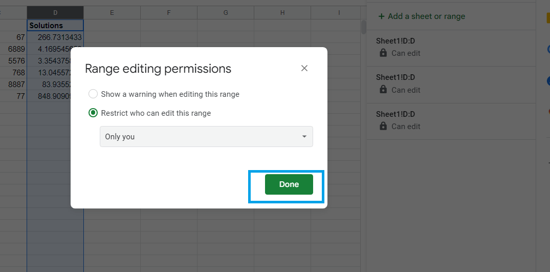 |
Step 7: Now, the selected range (column D) will be protected from editing, and other users will not be able to edit the column endless permitted.
 |
Conclusion
In conclusion, we have learned how to protect a specific cell range in Google sheets. Using this method, you can prevent the sheets from being accidentally, intentionally, or unauthorized edited by the users who have been granted editing permissions
Keywords: Google Docs, Google Sheet, How to Protect cells using Protect sheets and Ranges in Google Sheets