How do you freeze rows and columns in Google Sheets

Published June 12, 2022

With Google Sheets, you can store and organize enormous quantities of data in one spreadsheet. As a matter of fact, Google Sheets allows you to display thousands of rows of data at once! However, what if we need to keep a few of these rows and columns visible while scrolling through data?

The user-friendly spreadsheet overview in Google Sheets reduces the number of rows and columns displayed. It's inconvenient and time-consuming to have to continually scroll back and forth through your spreadsheet only to find some vital data. Fortunately, Google Sheets has an option for freezing rows and columns so we can examine selected sets of data.

In this article, we will cover the following topics:

How to freeze rows in Google sheets
How to freeze columns in Google sheets

How to freeze rows in Google sheets

It's quite easy to freeze a row, just follow the simple steps below:

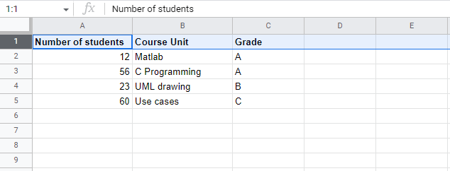
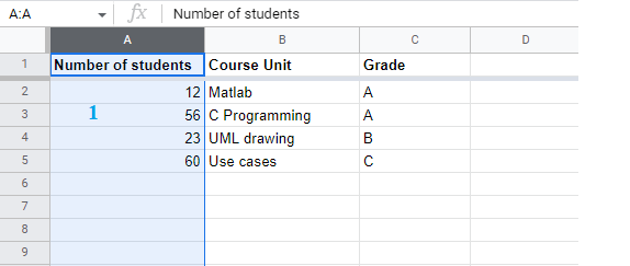
Step 1: Firstly, you need to identify the rows that you wish to freeze. For example, you can choose one row, two rows, or even three rows.

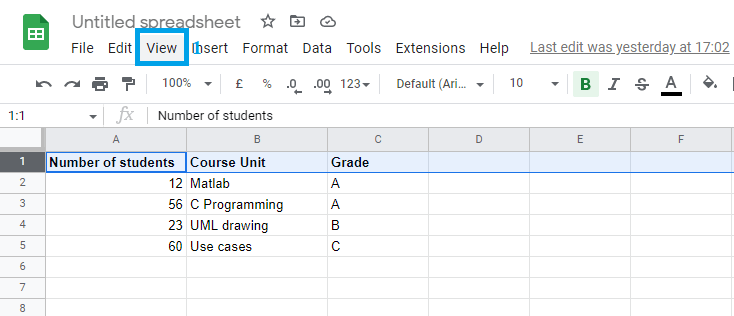
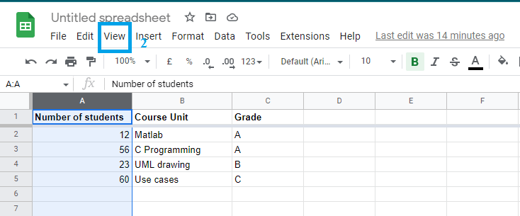
How do you freeze rows and columns in Google Sheets

Step 2: Now, on the Google sheets menu, click “View”

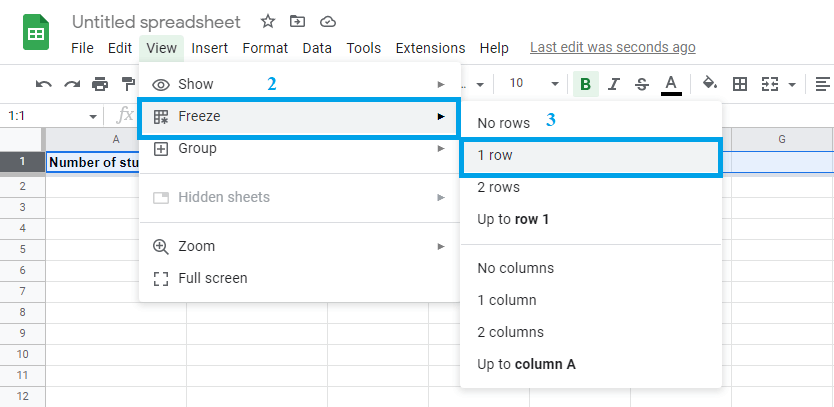
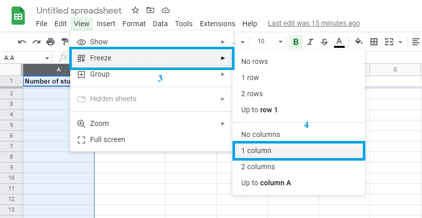
How do you freeze rows and columns in Google Sheets-2

Step 3: In the “View” submenu, select “freeze” and then specify the number of rows you would like to freeze. In our case, we will select “1 row”.

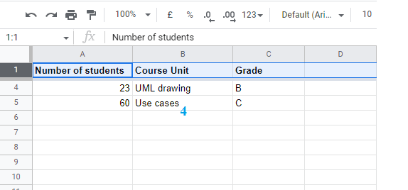
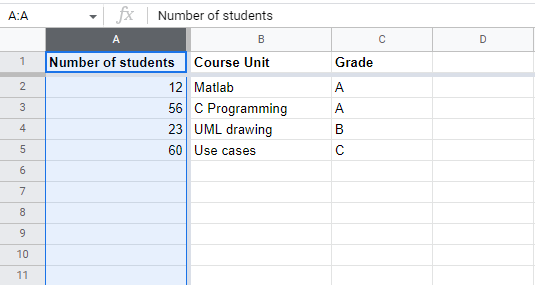
How do you freeze rows and columns in Google Sheets-3

Step 4: We are done freezing our row. The specified number of columns will be frozen, and if you scroll up or down, the row will remain visible at a fixed position.

How do you freeze rows and columns in Google Sheets-4

How to freeze columns in Google sheets

Here's how to freeze a column:

Step 1: First, specify the column or columns that you want to be frozen. In this tutorial, we will freeze the leftmost column.

How do you freeze rows and columns in Google Sheets-5

Step 2: Now, on the Google sheets menu, click "view"

How do you freeze rows and columns in Google Sheets-6

Step 3: On the “View” submenu, hover over “Freeze” and specify the number of columns you would like to freeze. In our case, we will select a single column.

How do you freeze rows and columns in Google Sheets-7

Step 4: We have frozen our selected column, and whenever you scroll right or left, it will remain at its current position.

How do you freeze rows and columns in Google Sheets-8

Conclusion

We have now learned how to freeze rows and columns. Alternatively, you can unfreeze the rows by clicking on view, hovering your cursor over freeze, and then selecting "No rows ."You can also unfreeze columns by clicking "View," hovering over "freeze," and selecting "No columns."

Keywords: Google Docs, Google Sheets, How to freeze rows and columns in Google Sheets

Related Google Sheet Question and Answers

How do i create new google sheet

How to delete a sheet in google sheet

How to duplicate google sheet

How to modify rows width columns and cells in google sheet

How to copy and paste cells in google sheet

How to drag and drop cells in google sheet

How to insert data using the fill handle the feature google sheet

How to insert,move and delete rows and columns google sheet

How to select cells in google sheet

How to freeze rows and columns google sheet